For my final project I wanted to look at US crime data from the FBI to see if there are gendered differences in arrest trends. Arrest numbers don’t necessarily reflect actual crime rates (because not all arrests result in convictions), but trends in arrest rates could roughly reflect trends in crime rates. I used the “Arrest Data – Reported Number of Adult Arrests by Crime” data set from the FBI Crime Data Explorer website.

To compare the rates of change in arrests I decided to use the Student’s t-test to compare the slopes of the year-by-year statistics for arrests by gender. The hypothesis tested was that the arrest rates were significantly different between genders, while the null hypothesis was that the arrest rate changes had similar trends between genders (p greater than 0.05).

The first step was to import the data into R, select the data I was interested in, then clean it up to make it easier to work with. The data set includes breakdowns of arrests by year, type of crime, gender, age group, and race. As I was focused on gender, I only kept the year, type of crime, gender, and arrest totals.

library("tidyr")
library("ggplot2")

# Read data on adult arrests downloaded from the FBI Crime Data Explorer:
# https://crime-data-explorer.fr.cloud.gov/downloads-and-docs
# Under "Arrest Data - Reported Number of Adult Arrests by Crime"
raw_crimedata <- read.csv("G:/arrests_national_adults.csv", header=TRUE)

# Extract the columns of interest to this project
gendersums <- raw_crimedata[,c("year", "offense_name", "total_male", "total_female")]
# Make gender a column to make the data easier to plot later
gendersums <- gather(gendersums, gender, total, c(total_male, total_female), factor_key=TRUE)
# Change the factor names in the new gender column to "male" and "female"
levels(gendersums$gender)[levels(gendersums$gender)=="total_male"] <- "male"
levels(gendersums$gender)[levels(gendersums$gender)=="total_female"] <- "female"

That gave me a data frame containing years, offense names, genders, and total arrests for a given year, gender, and offense combination.

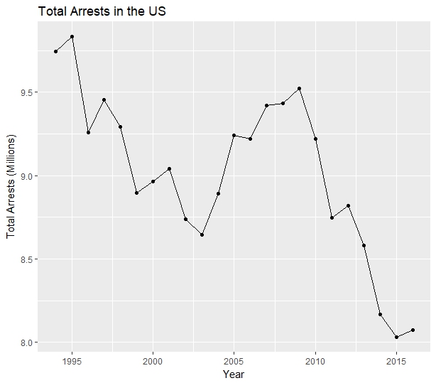
Before looking at the gender breakdown I checked the total arrests for all genders year-by-year.

# Get ungendered arrest totals
ungendered_totals <- aggregate(total ~ year, data=gendersums, FUN=sum)
# Plot ungendered arrest totals
ggplot(data=totals, aes(year, total / 1000000)) +
  geom_line() +
  geom_point() +
  labs(title="Total Arrests in the US", x = "Year", y = "Total Arrests (Millions)")

The resulting graph showed a general downward trend, with total arrests increasing from 2003 to 2009.

Next I created a data frame to hold the total arrests per gender, removing the distinction by offense type. Then I ran a t-test on the data to compare rates of change between male and female arrest totals.

# Get year-by-year totals of all crimes by gender
totals <- aggregate(total ~ year + gender, data=gendersums, FUN=sum)
# Run Student's t-test to compare the arrest totals by gender per year
t.test(total ~ gender, data=totals)

The output of the t-test was:

	Welch Two Sample t-test

data:  total by gender
t = 39.748, df = 26.498, p-value < 2.2e-16
alternative hypothesis: true difference in means is not equal to 0
95 percent confidence interval:
 4660622 5168465
sample estimates:
  mean in group male mean in group female
             6962686              2048142

The p value was extremely low – well below 0.05. For a p value of 0.05 the t value needed to be above approximately 1.7 to be considered significant – the t value was nearly 40. I concluded that the data did not support the null hypothesis, and that there were differences in the arrest rate changes between men and women year-to-year.

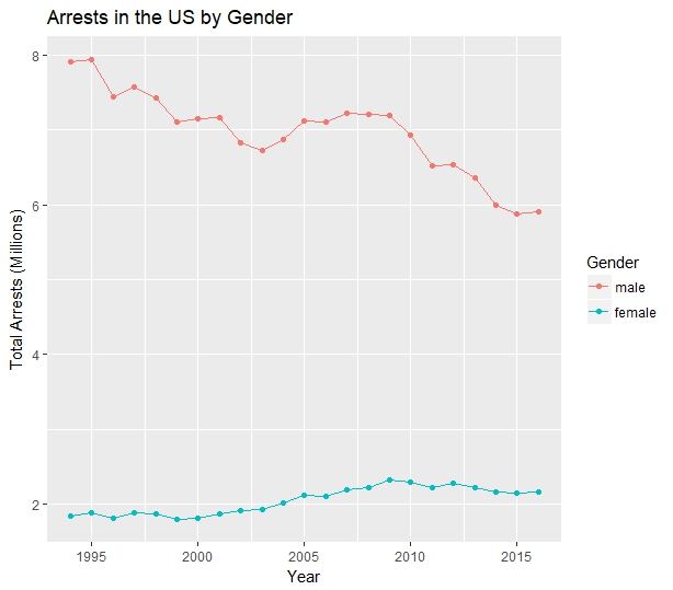
That conclusion is borne out by charting arrest totals for males and females and observing their slopes.

There’s a clear difference in the trends – arrest numbers have dropped for men since 1994, while arrest numbers for women have increased. Crunching the numbers, total arrests for men decreased by 25.2% from 1994 to 2016, while total arrests of women increased by 17.9% over the same period.

I was curious to see which offenses contributed the most to the difference between male and female arrests, so I went a step further in my analysis. I calculated the percentage changes in arrests for each offense type. Then, to narrow the list of offenses to those most likely to have had an impact on the figures, I selected only offenses for which there were more than 10,000 female arrests listed for 2016 and for which the gap between changes for the genders between 1994 and 2016 was greater than 50 percentage points.

The result indicated that the offenses that drove the relative changes in female arrests were burglary, driving under the influence, drug abuse violations, motor vehicle theft, simple assault, vandalism, and uncategorized offenses. I charted those offenses to show the percentage increase or decrease for both genders.

The results are interesting. Some offenses saw very large increases in female offenders (like drug offenses), while others are noteworthy for how much male arrests decreased (like car theft).

The code used to select the offenses to display on the chart above isn’t pretty, but it’s printed below.

# Calculate percentage change by offense type and gender
changes_list <- by(gendersums, gendersums[,"offense_name"], function(x) {
  (x[x$year==2016, "total"] - x[x$year==1994, "total"]) / x[x$year==1994, "total"] * 100
} )

# Make a flat vector of numbers so they can be moved to a data frame more easily
flat_changes <- unlist(changes_list)
# Assign genders to the calculated percentages, then build the data frame
male <- flat_changes[seq(1,length(flat_changes), 2)]
female <- flat_changes[seq(2,length(flat_changes), 2)]
offense <- names(changes_list)
changes <- data.frame(offense, male, female)
# Remove entries where the gap between male and female arrests is less than 50 percentage points
changes <- changes[changes$female - changes$male >50,]
# Make a data frame with 2016 entries where the number of female arrests was over 10k
high_female <- gendersums_wide[gendersums_wide$total_female > 10000 & gendersums_wide$year==2016,]
# Use the intersection of changes and high_female to select the most significantly changed offense types
changes <- changes[intersect(changes$offense, high_female$offense_name),]
changes <- gather(changes, gender, percent_change, c(male, female), factor_key=TRUE)
ggplot(data=changes) +
  geom_col(aes(x=offense, y=percent_change, fill=gender), position="dodge") +
  theme(axis.text.x = element_text(angle = 90, hjust = 1)) +
  labs(title="Change in Arrest Totals in the US from 1994 to 2016", x = "Offense", y = "Percentage Change", fill="Gender")

Thanks for an instructive semester!