Monthly Archives: February 2018

Module 7 – R Objects, S3 vs. S4

This week we looked at S3 and S4 objects in R.

My code for the exercise is on GitHub here:

https://github.com/jered0/lis4930-rpackage/blob/master/module7/s3s4objects.r

I used the trees dataset bundled with R for the exercise.

The trees dataset works with several generic functions, but not all. For example, summary(trees) returns:

     Girth           Height       Volume
 Min.   : 8.30   Min.   :63   Min.   :10.20
 1st Qu.:11.05   1st Qu.:72   1st Qu.:19.40
 Median :12.90   Median :76   Median :24.20
 Mean   :13.25   Mean   :76   Mean   :30.17
 3rd Qu.:15.25   3rd Qu.:80   3rd Qu.:37.30
 Max.   :20.60   Max.   :87   Max.   :77.00

However, mean(trees) doesn’t work because trees is a list, not a numeric vector.

The trees dataset can be used with both S3 and S4 functions. The data is straightforward (three numerical values per row), so it works well with both an S3-style list and as distinct values in an S4 class. In my code for the exercise I define both S3 and S4 classes that can contain records from the trees dataset, including a print() function for the S3 class and a show() function for the S4 class, and use apply() to map the dataset to each objects from each class.

Exercise questions

1. How do you tell what OO system (S3 vs. S4) an object is associated with?

You can check which class system was used to create an object using the otype() function from the “pryr” library. For example, the following command, using the S4 class from my exercise code, would yield a result of “S4″:

otype(new("trees_s4", Girth=1, Height=2, Volume=3))

2. How do you determine the base type (like integer or list) of an object?

You can determine the base type of an object with the mode() function. Running mode(trees) will show that the trees dataset is a list, for example, while mode(1) will show that 1 is a numeric type.

3. What is a generic function?

A generic function is a function that can be implemented in different ways for each class but called with a generic dispatcher. Calling the generic print() method, for example, will cause the interpreter to check the class of the object in question for its own implementation of print(). Generic functions offer a uniform interface that can be used without regard for implementation.

4. What are the main differences between S3 and S4?

An S3 class is essentially a list with a class attribute. That makes the implementation very flexible, as it’s not picky about how objects are defined and used. Code can add more items to a particular object’s list without a problem.

An S4 class is less flexible, requiring that the fields on an object be limited to those established in its class definition. Fields in an S4 class are also strictly typed, throwing an error if a value of the wrong type is assigned to them.

An S4 class is not as flexible as an S3 class because it’s not a list – it’s a defined class. While that stricter implementation is more inhibiting than an S3 class, the well-defined type checking can prevent unexpected errors in code using an S4 class.
Posted in R Programming | Comments Off

Module 5: JavaScript Form Validation and Wireframe Design

For the web programming portion of this week’s assignment, students were asked to create a form that would validate input using JavaScript. The web page with the form code is here:

Module 5 web page

Deciding to try to validate the email caused me the most trouble – mostly because I tried putting quotes around the regular expression at first. That was clearly a mistake.

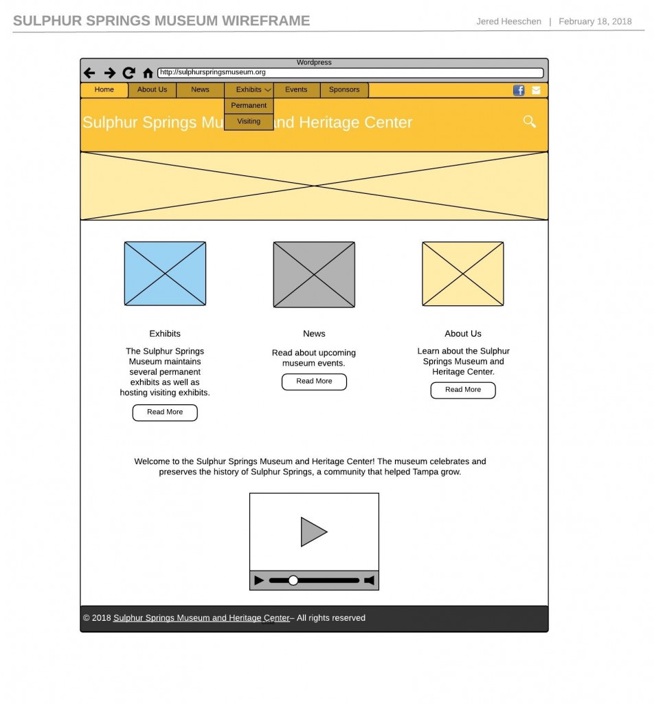
For the web design portion of the assignment, students were asked to create a wireframe of a website.

I’m working on a website for the Sulphur Springs Museum for my Senior Capstone project, so I created a wireframe of the site redesign so far. This should be useful for me as I can move elements around and tweak them to see what works before implementing it on the new site.

I used LucidChart to make the wireframe – they offer free accounts to students, and I’ve used the site before.

The wireframe is embedded here (click to enlarge):

Wireframe of the proposed website redesign for the Sulphur Springs Museum

You can also view it on the LucidChart website for a closer look.

The goal of the newer site design is to use a more modern aesthetic than what they have now. The top bar will have menus to navigate the site and links to email the museum or visit their Facebook page. Below that is the title of the site, with a search button to the right. Below that will be a rolling image bar that will display images from Sulphur Springs, both historically and modern-day.

Below the rolling image eye-catcher will be images that link to the major informational sections of the site – a list of exhibits, museum news, and a page providing background about the museum. Then at the bottom of the page is a video about the museum – I might change that presentation, for now the video is there to mimic that part of the current site’s design. I plan to replace the video with a map and photo of the museum, then, but don’t want to do that until I talk to the museum director about that design choice.

I wanted to keep the landing page fairly uncluttered overall – the pages with more content will include a sidebar listing recent posts, a calendar of upcoming events, and a link to Google Maps. I feel like a simple landing page will focus people on the elements that would be more likely to hold their attention (like the exhibits), then the pages after that can present more information.

Posted in Web Design Technologies | Comments Off

Module 6 – Matrix math and simulations in R Part 2

The assignment this week involved performing math with matrices, building a matrix with diag(), and generating a specific matrix.

The code for my solution is on github here:

https://github.com/jered0/lis4930-rpackage/blob/master/module6/matrices2.r

The first part was straightforward – A + B…

     [,1] [,2]
[1,]    7    5
[2,]    2    2

…and A - B:

     [,1] [,2]
[1,]   -3   -3
[2,]   -2    4

Next we were to generate a 4×4 matrix with a diagonal of (4, 1, 2, 3). After poking around with the diag() command, that turned out to be a one-line command:

diag(c(4, 1, 2, 3))

With the result:

     [,1] [,2] [,3] [,4]
[1,]    4    0    0    0
[2,]    0    1    0    0
[3,]    0    0    2    0
[4,]    0    0    0    3

Finally, we were to create a specific matrix:

     [,1] [,2] [,3] [,4] [,5]
[1,]    3    1    1    1    1
[2,]    2    3    0    0    0
[3,]    2    0    3    0    0
[4,]    2    0    0    3    0
[5,]    2    0    0    0    3

I started out by using integer(25) to create an empty matrix, but had overlooked the hint in the question suggesting that I use diag() to create the matrix instead. That made for more compact code, so I made the matrix using a combination of diag() and rep(). Then I wrote the last 4 entries in the first row with all 1s, and the last 4 entries in column 1 with all 2s, again using rep(). The code looked like this:

C <- diag(rep.int(3, 5))
C[1,2:5] <- rep.int(1, 4)
C[2:5,1] <- rep.int(2, 4)
Posted in R Programming | Comments Off

Module 5: Doing Matrix Math in R

The assignment this week was to create two matrices and calculate their inverses and their determinants. The values given were:

A=matrix(1:100, nrow=6)
B=matrix(1:1000, nrow=6)

Unfortunately, those values don’t work – a matrix has to have a number of values that can be translated into a matrix given the number of rows, and you can’t divide 6 evenly into either 100 or 1000. To remedy this, I changed the number of rows for each matrix from 6 to 10.

The R commands I used were:

A <- matrix(1:100, nrow=10)
B <- matrix(1:1000, nrow=10)

The R command to find the inverse is solve(), so next I ran that command on the two matrices.

And…that didn’t work out so well. The error message told me that A was singular, so it didn’t have an inverse. And B wasn’t square, so it couldn’t have an inverse either.

The determinant is found with the det() function, so I tried that out too. The determinant of A was 0 (makes sense, given the result I got trying to get the inverse), and then B threw an error because it couldn’t get the determinant of a matrix that wasn’t square. Foiled again.

So I dug into random numbers to generate a non-sequential set of numbers for a new matrix. And I wanted the result to be repeatable (to make it easier to replicate and grade), so I used set.seed() and runif(). I also focused only on A, because I couldn’t make a square matrix out of 1000 numbers. Sorry, B.

set.seed(123)
A <- matrix(runif(100, min=1, max=100), nrow=10)

That made A into:

           [,1]      [,2]     [,3]      [,4]     [,5]      [,6]     [,7]      [,8]     [,9]    [,10]
 [1,] 29.470174 95.726501 89.06439 96.339399 15.13720  5.537286 66.84640 75.693041 25.11833 13.93887
 [2,] 79.042208 45.880081 69.58754 90.327605 42.04009 44.777807 10.38923 63.292892 67.13750 65.65709
 [3,] 41.488715 68.079493 64.41017 69.379823 41.95871 80.093560 39.01299 71.308058 42.34703 35.00813
 [4,] 88.418723 57.690707 99.43271 79.751274 37.51570 13.068027 28.16398  1.061853 79.03139 66.01905
 [5,] 94.106261 11.189544 65.91487  3.436755 16.09203 56.533850 81.64936 48.056341 11.18360 32.71695
 [6,]  5.510093 90.082672 71.14452 48.301801 14.74180 21.446608 45.40312 22.791770 44.05438 19.58142
 [7,] 53.282443 25.362686 54.86254 76.087494 24.07038 13.625633 81.19637 38.601837 98.51074 78.44714
 [8,] 89.349485  5.163894 59.82006 22.424386 47.13028 75.577479 81.42656 61.664329 89.41206 10.26590
 [9,] 55.592066 33.464151 29.62681 32.499920 27.33129 89.609491 79.63989 35.827993 88.76044 47.21113
[10,] 46.204859 95.495861 15.56425 23.930953 85.92494 38.071815 44.54334 12.002407 18.33021 51.63904

Now I could get the inverse and determinant:

solve(A)
det(A)

The determinant was returned as 2.471786e+18. The inverse was:

              [,1]         [,2]         [,3]         [,4]          [,5]         [,6]          [,7]          [,8]         [,9]         [,10]
 [1,]  0.012404331  0.014655568 -0.024950989  0.002363324  0.0024883203 -0.007528454 -0.0155334345 -0.0006610557  0.016073655  0.0022233330
 [2,]  0.005498005  0.018905283 -0.025300934 -0.008300409  0.0010619645  0.014340780 -0.0126398624 -0.0031970118  0.012703786  0.0043549557
 [3,] -0.013711628 -0.010417761  0.019364467  0.004667232  0.0055394390  0.012004889  0.0086199292  0.0039862656 -0.020829129 -0.0050540560
 [4,]  0.016471142 -0.022182260  0.020340061  0.019413907 -0.0105374733 -0.033021567 -0.0004251472 -0.0056725764  0.009574390 -0.0026334849
 [5,] -0.007553095 -0.017673061  0.024248454  0.005571115 -0.0059687886 -0.008097359  0.0116419862  0.0105975716 -0.021416142  0.0075871860
 [6,] -0.002072423 -0.011888989  0.018786337  0.007942099 -0.0007145655 -0.008617087 -0.0040702093 -0.0047360911  0.007951269 -0.0036383211
 [7,]  0.006674229 -0.018906014  0.008345737  0.005219274  0.0007914594 -0.011320821  0.0069961331 -0.0008031338  0.002070228  0.0013363260
 [8,] -0.003758705  0.025465328 -0.015070004 -0.022802631  0.0051107692  0.017684411  0.0024590013  0.0049765108 -0.008003417  0.0006537543
 [9,] -0.003791975  0.014823496 -0.017791253 -0.007537918 -0.0051919999  0.015235601 -0.0016023448  0.0075767455  0.003805645 -0.0011647558
[10,] -0.014208379  0.008644982  0.002271745 -0.008820289  0.0094544005  0.011974071  0.0124641286 -0.0093644472 -0.007537431  0.0012324687

The code for my program is here:

https://github.com/jered0/lis4930-rpackage/blob/master/module5/matrixinverse.r

Posted in R Programming | Comments Off

Module 4 – JavaScript Conditional Statements

The assignment was in two parts – write JavaScript that tested two conditions with AND in an if statement, and save an image in different formats to see how they compared.

The webpage with the JavaScript and images is here:

http://jered.0fees.us/module4/

The JavaScript was similar to working with if/else statements in other languages, apart from the loose typing – being able to toss a number and a string into the same variable, for example, then test them, was different from Java. I also put the test into a function and called it twice, for fun.

For the image, I took a large JPG file, reduced the dimensions to 1022×576, then converted it to GIF, JPG, PNG 8-bit, and PNG 24-bit. The 24-bit PNG was the largest file at 905k, the 8-bit PNG was the smallest at 259k, and the GIF and JPG were close to each other in size – 361k and 367k, respectively.

The image quality of the resulting images was pretty similar to my naked eye. At first glance, the images aren’t too different.

Looking closely, the GIF image’s limited number of colors don’t handle shadows and shades of white very well – there isn’t a smooth progression from one shade to the next. The eyes on the pottery especially have that problem.

The other three formats looked similar to each other. I expected the 8-bit PNG to look more like the GIF file, but I wasn’t able to pick out significant differences between it and the JPG and PNG-24, to be honest.

Posted in Web Design Technologies | Comments Off

R Module 4 – R Programming Structure

This week’s assignment was to create a boxplot graph and a histogram from a set of patient data. The full program is here:

https://github.com/jered0/lis4930-rpackage/blob/master/module4/patientdata.r

I wanted to use the data as presented (changing a couple curly-quotes to straight quotes), then convert it within the program into numeric data that could be plotted. It was more work than expected, and it’s possible it could have been done more efficiently than I wound up doing it.

The first big obstacle was converting text to numeric values. I worked it out using ifelse() to convert the text values.

The other big obstacle involved the data types being used. When I created a data frame with the values, it turned the values into “factor” types, which couldn’t be plotted. Converting some of the numbers into a numeric type directly resulted in strange values, so to work around that I converted the values to characters first, then to the numeric type.

I also went overboard on the boxplot. Looking for ways to make it useful to a doctor reviewing it, I wanted to use the boxplot itself to show the average of the two doctors’ opinions on the patient condition. To make that more meaningful, I plotted two other values as points on that graph – one for the ER priority assigned to the patient (so doctor opinions could be contrasted with the patient’s ER condition), and one for blood pressure (so a doctor could see whether there was a correlation between BP and patient condition).

Then I had to learn how to use a legend, because it felt wrong putting so many colored dots on the graph without a legend to explain them.

The histogram, by comparison, was straightforward – I plotted only one value (frequency of patient visits) so doctors could see how frequently patients tended to come in for examinations. Then it was just a matter of setting axis labels and such.

Posted in R Programming | Comments Off