This week we looked at random variables and probability distributions.

The first assignment was to take two sets of values and their probabilities and determining the standard deviation for both.

The R code I used for the first set is:

t1 <- data.frame(x=c(0, 1, 2, 3), p=c(0.5, 0.2, 0.15, 0.10))
t1mu <- sum(t1$x * t1$p)
t1var <- sum((t1$x - t1mu)^2 * t1$p)
t1sd <- sqrt(t1var)
t1sd

The standard deviation was reported as 1.013903.

The code for the second set was:

t2 <- data.frame(x=c(1, 3, 5, 4), p=c(0.10, 0.2, 0.6, 0.2))
t2mu <- sum(t2$x * t2$p)
t2var <- sum((t2$x - t2mu)^2 * t2$p)
t2sd <- sqrt(t2var)
t2sd

The standard deviation for the second set was 1.369306.

The standard deviation was higher for the second set, probably because the second set had a high probability attached to its largest value, and the range was higher for the second set as well.

The second part of the assignment called for finding p(x=0) for a binomial distribution where the number of trials was 4 and the probability of success was 0.12.

The code I used to solve the problem was:

dbinom(0, 4, 0.12)

The result for p(0) was 0.5996954.

The final part of the assignment called for the creation of 20 Poisson numbers and calculating the value of the mean and the variance of the results. Lambda wasn’t provided, so I used 3 for the value. The code I ran was:

poisvec <- rpois(20, 3)
mean(poisvec)
var(poisvec)

I ran the code a few times to see how much it would vary. The expected mean and variance would be around 3 because that’s the point of Poisson variables – lambda represents the target mean and variance.

The first run I got a mean of 2.8 and a variance of 3.22. The second time I got a mean of 3.2 and a variance of 4.69. The third run I got a mean of 3.05 and a variance of 2.16.

Generating 20 values allowed for a good deal of variety in the variance, apparently.

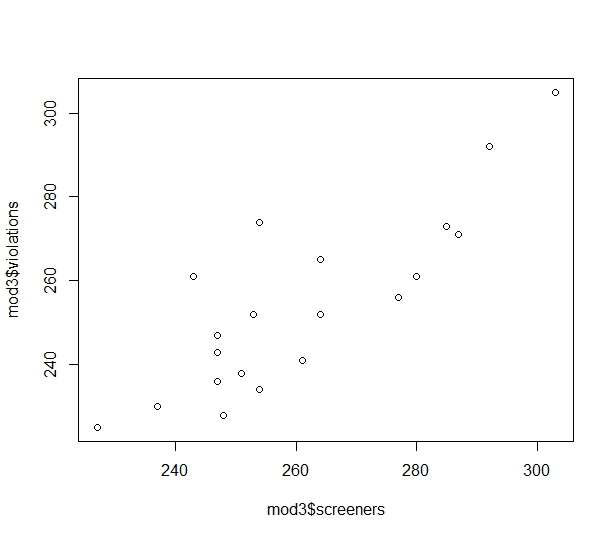
The assignment this week involved examining a data set of pre-boarding screener turnover and security violations detected at US airports between 1988 and 1999. The instructor selection 20 data points at random and asked us to check for correlations.

The first task was to describe the association between the screener data and violations data. Based on the number crunching in the questions that followed, it appears that there was a fairly strong positive correlation between screener turnover and the number of security violations detected.

The next tasks involved calculating the Pearson’s sample correlation coefficient and the Spearman’s rank coefficient, then to create a scatterplot of the data. The code for those tasks follows (after importing the data from the assignment page into my RStudio workspace):

cor.test(mod3$screeners, mod3$violations)
cor.test(mod3$screeners, mod3$violations, method="spearman")
plot(mod3$screeners, mod3$violations)

Pearson’s coefficient: 0.8375321

Spearman’s coefficient (rho): 0.7575423

Scatterplot:

It turns out I’m too late posting this to get credit, but I’ll post it anyway because the work is done. Note to self: remember to check due time as well as due date.

The assignment was to find various calculations for two vectors then compare them. My code:

x <- c(10, 2, 3, 2, 4, 2, 5)
y <- c(20, 12, 13, 12, 14, 12, 15)

# Took function to find the mode from:
# https://stackoverflow.com/a/8189441
# The mode() function reports a values type (like "numeric")
get_mode <- function(x) {
  ux <- unique(x)
  ux[which.max(tabulate(match(x, ux)))]
}

get_cv <- function(x) {
  sd(x) / mean(x) * 100
}

cat("For X, mean:", mean(x), "median:", median(x), "mode:", get_mode(x), "\n")
cat("For Y, mean:", mean(y), "median:", median(y), "mode:", get_mode(y), "\n")

cat("--\n")

# Assuming that the question was for quantile, given that was the function
# described - otherwise I'd use the IQR() function to find interquartile range
cat("For X, range:", range(x), "quantile:", quantile(x), "variance:", get_cv(x), "standard deviation:", sd(x), "\n")
cat("For Y, range:", range(y), "quantile:", quantile(y), "variance:", get_cv(y), "standard deviation:", sd(y), "\n")

The result:

For X, mean: 4 median: 3 mode: 2
For Y, mean: 14 median: 13 mode: 12
--
For X, range: 2 10 quantile: 2 2 3 4.5 10 variance: 72.16878 standard deviation: 2.886751
For Y, range: 12 20 quantile: 12 12 13 14.5 20 variance: 20.61965 standard deviation: 2.886751

The most interesting result when comparing the two datasets was that the standard deviance was identical for both sets, despite the ranges and variances being very different.

The assignment was straightforward, mostly because of previous courses using R – I’ve used these functions before, apart from variance and the custom mode function I picked up from the Internet.