Our assignment this week was to debug a block of code.

The original code was:

tukey_multiple <- function(x) {
   outliers <- array(TRUE,dim=dim(x))
   for (j in 1:ncol(x))
    {
    outliers[,j] <- outliers[,j] && tukey.outlier(x[,j])
    }
outlier.vec <- vector(length=nrow(x))
    for (i in 1:nrow(x))
    { outlier.vec[i] <- all(outliers[i,]) } return(outlier.vec) }

To start debugging, I pasted the code into RStudio to see what kind of error it would throw. I got:

Error: unexpected symbol in:
"    for (i in 1:nrow(x))
    { outlier.vec[i] <- all(outliers[i,]) } return"

The “unexpected symbol” error made me think that some brackets or parentheses weren’t closed or were misplaced. That wasn’t it, but it turned out to be something similar – looking at the last line, I noticed that the “return” looked out of place. It should have been on a separate line, by itself. That would certainly make it an unexpected symbol. I moved return to the next line, making the code look like:

tukey_multiple <- function(x) {
  outliers <- array(TRUE,dim=dim(x))
  for (j in 1:ncol(x))
  {
    outliers[,j] <- outliers[,j] && tukey.outlier(x[,j])
  }
  outlier.vec <- vector(length=nrow(x))
  for (i in 1:nrow(x))
  { outlier.vec[i] <- all(outliers[i,]) }
  return(outlier.vec) }

At that point, the code ran successfully and the function was created.

Using the function was a different story – I passed it a built-in list as an argument, and got a new error:

Error in tukey.outlier(x[, j]) : could not find function "tukey.outlier"

I’m guessing that tukey.outlier() is a function that returns TRUE or FALSE depending on whether the value is an outlier. The code runs fine without that function (albeit it makes tukey.multiple() always return a bunch of TRUEs), so I assume this code will work provided tukey.outlier() is defined.

This week’s assignment was to create a DESCRIPTION file for our final project package.

The DESCRIPTION file I created is on GitHub here:

https://github.com/jered0/lis4930-rpackage/blob/master/queryNIBRS/DESCRIPTION

Getting the DESCRIPTION format right was interesting, and I ended up looking at a few packages on CRAN to see what package names typically look like and how they describe themselves. For example, I thought at first that the Title field was just an expanded name for the package, but I see that it does, as you said in the module, act more as a descriptive subtitle.

Because my package will involve retrieving data from the FBI’s Crime Data API, I added an Imports section for the dependency the package will need, RCurl. I’ll look into whether that’s strictly required – I might be able to use R’s built-in web queries instead of relying on RCurl’s fancy capabilities.

This week the assignment was to plot graphs for a data set using a built-in R function, a function from the lattice package, and a function from the ggplot2 package.

The source code I created for the task can be found on GitHub here:

https://github.com/jered0/lis4930-rpackage/blob/master/module9/lattice-ggplotting.r

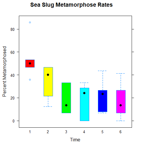
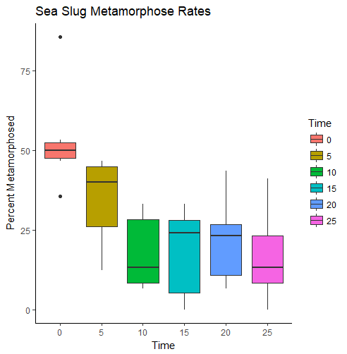
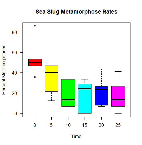
I used the SeaSlugs data set. A description of the set is on this page, and the data set itself can be downloaded via this link.

Given that there were two categories of data (time and metamorphose percentage), and there were multiple percentages for each time entry, I decided to represent the data with a boxplot.

Built-in function

I used the built-in boxplot() function to create the first graph.

I’ve used this function before, but I did have to fiddle with it to work out how to get the y-axis labels horizontal (I thought it looked better that way), and to apply colors from the rainbow() function. It’s a simple graph, nothing fancy.

Lattice function

I used the bwplot() function from the lattice package to make the next box plot graph.

The syntax is pretty close to the built-in function, which made it easier to work with than I expected. I had to tweak settings to get it to use vertical boxes, and had to find the parameter that would set the colors. Unfortunately I didn’t find an option to draw a line instead of use a plot to mark the median, to match the appearance of the other graphs.

ggplot2 function

For the final graph, I used the ggplot2 package’s ggplot(), geom_boxplot(), labs(), and theme_classic() functions in concert.

It took some time to get the syntax and everything sorted out, since it uses a different syntax from the other two functions. I also had to convert the Time column to factors – without that change, all the percentage data and time data were collected into one giant boxplot. Definitely not what I wanted.

The ggplot2 graph came out looking the best, I think, and next time there would be less fuss given that I’m more familiar with the package.

This module’s assignment was to read data from a file, alter or filter that data, then write the new data to new files.

The code I used is on my GitHub repository here:

https://github.com/jered0/lis4930-rpackage/blob/master/module8/studentsorting.r

I was generally familiar with the concepts involved in reading from files thanks to other coding languages, and the format of read.table is pretty intuitive, so I had no problems there. The file.chooser() function was easy to use, and being able to read the data in all at once without looping through lines one at a time was nice.

It did take me a bit to wrap my head around the ddply function, but running it a few times and tweaking the parameters cleared it up. Being able to fiddle with a data set and pick it apart like that definitely seems like it would come in handy.

I’ve used the grep command on Unix often, so using grepl() was straightforward – though I did have to look over the documentation to see how grep() and grepl() differ, and why grepl needed to be used with subset().

This week we looked at S3 and S4 objects in R.

My code for the exercise is on GitHub here:

https://github.com/jered0/lis4930-rpackage/blob/master/module7/s3s4objects.r

I used the trees dataset bundled with R for the exercise.

The trees dataset works with several generic functions, but not all. For example, summary(trees) returns:

     Girth           Height       Volume
 Min.   : 8.30   Min.   :63   Min.   :10.20
 1st Qu.:11.05   1st Qu.:72   1st Qu.:19.40
 Median :12.90   Median :76   Median :24.20
 Mean   :13.25   Mean   :76   Mean   :30.17
 3rd Qu.:15.25   3rd Qu.:80   3rd Qu.:37.30
 Max.   :20.60   Max.   :87   Max.   :77.00

However, mean(trees) doesn’t work because trees is a list, not a numeric vector.

The trees dataset can be used with both S3 and S4 functions. The data is straightforward (three numerical values per row), so it works well with both an S3-style list and as distinct values in an S4 class. In my code for the exercise I define both S3 and S4 classes that can contain records from the trees dataset, including a print() function for the S3 class and a show() function for the S4 class, and use apply() to map the dataset to each objects from each class.

Exercise questions

1. How do you tell what OO system (S3 vs. S4) an object is associated with?

You can check which class system was used to create an object using the otype() function from the “pryr” library. For example, the following command, using the S4 class from my exercise code, would yield a result of “S4″:

otype(new("trees_s4", Girth=1, Height=2, Volume=3))

2. How do you determine the base type (like integer or list) of an object?

You can determine the base type of an object with the mode() function. Running mode(trees) will show that the trees dataset is a list, for example, while mode(1) will show that 1 is a numeric type.

3. What is a generic function?

A generic function is a function that can be implemented in different ways for each class but called with a generic dispatcher. Calling the generic print() method, for example, will cause the interpreter to check the class of the object in question for its own implementation of print(). Generic functions offer a uniform interface that can be used without regard for implementation.

4. What are the main differences between S3 and S4?

An S3 class is essentially a list with a class attribute. That makes the implementation very flexible, as it’s not picky about how objects are defined and used. Code can add more items to a particular object’s list without a problem.

An S4 class is less flexible, requiring that the fields on an object be limited to those established in its class definition. Fields in an S4 class are also strictly typed, throwing an error if a value of the wrong type is assigned to them.

An S4 class is not as flexible as an S3 class because it’s not a list – it’s a defined class. While that stricter implementation is more inhibiting than an S3 class, the well-defined type checking can prevent unexpected errors in code using an S4 class.

The assignment this week involved performing math with matrices, building a matrix with diag(), and generating a specific matrix.

The code for my solution is on github here:

https://github.com/jered0/lis4930-rpackage/blob/master/module6/matrices2.r

The first part was straightforward – A + B…

     [,1] [,2]
[1,]    7    5
[2,]    2    2

…and A - B:

     [,1] [,2]
[1,]   -3   -3
[2,]   -2    4

Next we were to generate a 4×4 matrix with a diagonal of (4, 1, 2, 3). After poking around with the diag() command, that turned out to be a one-line command:

diag(c(4, 1, 2, 3))

With the result:

     [,1] [,2] [,3] [,4]
[1,]    4    0    0    0
[2,]    0    1    0    0
[3,]    0    0    2    0
[4,]    0    0    0    3

Finally, we were to create a specific matrix:

     [,1] [,2] [,3] [,4] [,5]
[1,]    3    1    1    1    1
[2,]    2    3    0    0    0
[3,]    2    0    3    0    0
[4,]    2    0    0    3    0
[5,]    2    0    0    0    3

I started out by using integer(25) to create an empty matrix, but had overlooked the hint in the question suggesting that I use diag() to create the matrix instead. That made for more compact code, so I made the matrix using a combination of diag() and rep(). Then I wrote the last 4 entries in the first row with all 1s, and the last 4 entries in column 1 with all 2s, again using rep(). The code looked like this:

C <- diag(rep.int(3, 5))
C[1,2:5] <- rep.int(1, 4)
C[2:5,1] <- rep.int(2, 4)

The assignment this week was to create two matrices and calculate their inverses and their determinants. The values given were:

A=matrix(1:100, nrow=6)
B=matrix(1:1000, nrow=6)

Unfortunately, those values don’t work – a matrix has to have a number of values that can be translated into a matrix given the number of rows, and you can’t divide 6 evenly into either 100 or 1000. To remedy this, I changed the number of rows for each matrix from 6 to 10.

The R commands I used were:

A <- matrix(1:100, nrow=10)
B <- matrix(1:1000, nrow=10)

The R command to find the inverse is solve(), so next I ran that command on the two matrices.

And…that didn’t work out so well. The error message told me that A was singular, so it didn’t have an inverse. And B wasn’t square, so it couldn’t have an inverse either.

The determinant is found with the det() function, so I tried that out too. The determinant of A was 0 (makes sense, given the result I got trying to get the inverse), and then B threw an error because it couldn’t get the determinant of a matrix that wasn’t square. Foiled again.

So I dug into random numbers to generate a non-sequential set of numbers for a new matrix. And I wanted the result to be repeatable (to make it easier to replicate and grade), so I used set.seed() and runif(). I also focused only on A, because I couldn’t make a square matrix out of 1000 numbers. Sorry, B.

set.seed(123)
A <- matrix(runif(100, min=1, max=100), nrow=10)

That made A into:

           [,1]      [,2]     [,3]      [,4]     [,5]      [,6]     [,7]      [,8]     [,9]    [,10]
 [1,] 29.470174 95.726501 89.06439 96.339399 15.13720  5.537286 66.84640 75.693041 25.11833 13.93887
 [2,] 79.042208 45.880081 69.58754 90.327605 42.04009 44.777807 10.38923 63.292892 67.13750 65.65709
 [3,] 41.488715 68.079493 64.41017 69.379823 41.95871 80.093560 39.01299 71.308058 42.34703 35.00813
 [4,] 88.418723 57.690707 99.43271 79.751274 37.51570 13.068027 28.16398  1.061853 79.03139 66.01905
 [5,] 94.106261 11.189544 65.91487  3.436755 16.09203 56.533850 81.64936 48.056341 11.18360 32.71695
 [6,]  5.510093 90.082672 71.14452 48.301801 14.74180 21.446608 45.40312 22.791770 44.05438 19.58142
 [7,] 53.282443 25.362686 54.86254 76.087494 24.07038 13.625633 81.19637 38.601837 98.51074 78.44714
 [8,] 89.349485  5.163894 59.82006 22.424386 47.13028 75.577479 81.42656 61.664329 89.41206 10.26590
 [9,] 55.592066 33.464151 29.62681 32.499920 27.33129 89.609491 79.63989 35.827993 88.76044 47.21113
[10,] 46.204859 95.495861 15.56425 23.930953 85.92494 38.071815 44.54334 12.002407 18.33021 51.63904

Now I could get the inverse and determinant:

solve(A)
det(A)

The determinant was returned as 2.471786e+18. The inverse was:

              [,1]         [,2]         [,3]         [,4]          [,5]         [,6]          [,7]          [,8]         [,9]         [,10]
 [1,]  0.012404331  0.014655568 -0.024950989  0.002363324  0.0024883203 -0.007528454 -0.0155334345 -0.0006610557  0.016073655  0.0022233330
 [2,]  0.005498005  0.018905283 -0.025300934 -0.008300409  0.0010619645  0.014340780 -0.0126398624 -0.0031970118  0.012703786  0.0043549557
 [3,] -0.013711628 -0.010417761  0.019364467  0.004667232  0.0055394390  0.012004889  0.0086199292  0.0039862656 -0.020829129 -0.0050540560
 [4,]  0.016471142 -0.022182260  0.020340061  0.019413907 -0.0105374733 -0.033021567 -0.0004251472 -0.0056725764  0.009574390 -0.0026334849
 [5,] -0.007553095 -0.017673061  0.024248454  0.005571115 -0.0059687886 -0.008097359  0.0116419862  0.0105975716 -0.021416142  0.0075871860
 [6,] -0.002072423 -0.011888989  0.018786337  0.007942099 -0.0007145655 -0.008617087 -0.0040702093 -0.0047360911  0.007951269 -0.0036383211
 [7,]  0.006674229 -0.018906014  0.008345737  0.005219274  0.0007914594 -0.011320821  0.0069961331 -0.0008031338  0.002070228  0.0013363260
 [8,] -0.003758705  0.025465328 -0.015070004 -0.022802631  0.0051107692  0.017684411  0.0024590013  0.0049765108 -0.008003417  0.0006537543
 [9,] -0.003791975  0.014823496 -0.017791253 -0.007537918 -0.0051919999  0.015235601 -0.0016023448  0.0075767455  0.003805645 -0.0011647558
[10,] -0.014208379  0.008644982  0.002271745 -0.008820289  0.0094544005  0.011974071  0.0124641286 -0.0093644472 -0.007537431  0.0012324687

The code for my program is here:

https://github.com/jered0/lis4930-rpackage/blob/master/module5/matrixinverse.r

This week’s assignment was to create a boxplot graph and a histogram from a set of patient data. The full program is here:

https://github.com/jered0/lis4930-rpackage/blob/master/module4/patientdata.r

I wanted to use the data as presented (changing a couple curly-quotes to straight quotes), then convert it within the program into numeric data that could be plotted. It was more work than expected, and it’s possible it could have been done more efficiently than I wound up doing it.

The first big obstacle was converting text to numeric values. I worked it out using ifelse() to convert the text values.

The other big obstacle involved the data types being used. When I created a data frame with the values, it turned the values into “factor” types, which couldn’t be plotted. Converting some of the numbers into a numeric type directly resulted in strange values, so to work around that I converted the values to characters first, then to the numeric type.

I also went overboard on the boxplot. Looking for ways to make it useful to a doctor reviewing it, I wanted to use the boxplot itself to show the average of the two doctors’ opinions on the patient condition. To make that more meaningful, I plotted two other values as points on that graph – one for the ER priority assigned to the patient (so doctor opinions could be contrasted with the patient’s ER condition), and one for blood pressure (so a doctor could see whether there was a correlation between BP and patient condition).

Then I had to learn how to use a legend, because it felt wrong putting so many colored dots on the graph without a legend to explain them.

The histogram, by comparison, was straightforward – I plotted only one value (frequency of patient visits) so doctors could see how frequently patients tended to come in for examinations. Then it was just a matter of setting axis labels and such.

The assignment was to take a set of data and perform operations on it as a data frame, per an example document.

The variables with the initial data were:

Name <- c("Jeb", "Donald", "Ted", "Marco", "Carly", "Hillary", "Berine")
ABC <- c(4, 62, 51, 21, 2, 14, 15)
CBS <- c(12, 75, 43, 19, 1, 21, 19)

I tried turning that into a matrix…

candidates.m <- cbind(Name, ABC, CBS)

…and got a matrix full of strings.

     Name      ABC  CBS
[1,] "Jeb"     "4"  "12"
[2,] "Donald"  "62" "75"
[3,] "Ted"     "51" "43"
[4,] "Marco"   "21" "19"
[5,] "Carly"   "2"  "1"
[6,] "Hillary" "14" "21"
[7,] "Berine"  "15" "19"

So I made a data frame from the data.

candidates.df <- data.frame(Name, ABC, CBS)

The resulting data frame:

     Name ABC CBS
1     Jeb   4  12
2  Donald  62  75
3     Ted  51  43
4   Marco  21  19
5   Carly   2   1
6 Hillary  14  21
7  Berine  15  19

I tried to run the mean command on the data frame, but it didn’t work out in RStudio the way it did in the example. The example showed an error for the text column and then means for the numeric columns, but all I got was the error.

> mean(candidates.df)
[1] NA
Warning message:
In mean.default(candidates.df) :
  argument is not numeric or logical: returning NA

I got the same error when specifying the two numeric columns.

mean(candidates.df[,2:3])

But I could get the mean of a specific column.

> mean(candidates.df[,2])
[1] 24.14286

To get the means of the columns I had to use colMeans on the numeric columns specifically – using colMeans on the full dataframe resulted in an error that “‘x’ must be numeric”.

colMeans(candidates.df[2:3])

Result:

     ABC      CBS
24.14286 27.14286

I could also use rowMeans to get means by row.

> rowMeans(candidates.df[2:3])
[1]  8.0 68.5 47.0 20.0  1.5 17.5 17.0

Using as.matrix(candidates.df) gave the same matrix as I listed at the top of this post.

Data frames are interesting as a means of storing mixed data in a matrix-like structure. It has its caveats when the columns have different modes, but those can be worked around with the right code.

In module 2, the class was asked to test and evaluate R code. We were given two commands:

assignment2 <- c(16, 18, 14, 22, 27, 17, 19, 17, 17, 22, 20, 22)
myMean <- function(assignment2) { return(sum(assignment)/length(someData)) }

The first line creates a dataset labeled assignment2, and the second line creates a function named myMean. Judging by the code, myMean is meant to calculate the mean of the dataset sent to it as an argument.

Unfortunately, the code doesn’t work as written, giving an object not found error. The problem lies in the variables used in the body of the function – neither assignment nor someData have been given values. If the goal is to find the mean of the dataset passed to the function as an argument, then the names of the variables in the function body should match that of the function’s argument.

The function works, then, if it’s rewritten as:

myMean <- function(assignment2) { return(sum(assignment2)/length(assignment2)) }

For clarity it might make sense to change the argument of the function to assignment instead of assignment2. That way there wouldn’t be a potential for confusion between the global variable and the internal variable processed by the function. Because of the scope difference, however, the identical names don’t create a problem for the result – passing a different dataset to the function causes it to return the mean of that dataset, not the dataset contained in the global assignment2 variable.